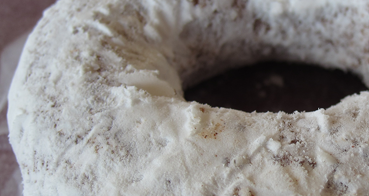
Having written yesterday about nanoparticle titanium dioxide (TiO2) concentrations in donuts, Raphaël Lévy asked for some clarification on where I got my figures from. I thought it easiest to post the analysis in full – it goes a little deep into particle analysis, but on the other hand it’s also a useful example of the level of particle size distribution analysis I rarely see in nanoparticle papers these days.
Preparing for the analysis
The starting point was the As You Sow reported analysis by Analytical Sciences LLC on the mass of TiO2 10 nm in diameter and below in the coatings on donuts. In any analysis, it’s good practice to test the data for “reasonableness” – i.e. whether they make sense or are utter nonsense. To do this, I first needed data on the typical size distribution of food grade TiO2 particles – the material that will have been used in the donut coatings.
There are a number of sources that I could have used here, but I chose to go with a recent paper published by Yang et al.:
Yu Yang, Kyle Doudrick, Xiangyu Bi, Kiril Hristovski, Pierre Herckes, Paul Westerhoff, and Ralf Kaegi (2014) Characterization of Food-Grade Titanium Dioxide: The Presence of Nanosized Particles Environ Sci Tech DOI: 10.1021/es500436x
This paper specifically reports on the particle size distribution from five samples of food grade TiO2, using Transmission Electron Microscopy Analysis. However, the way the data are presented (particle counts between specific particle diameters) isn’t sufficient on its own to estimate the likely mass of particles below 10 nm in a typical food grade TiO2 powder. For this, the usual approach is to represent the particle counts with a mathematical function that represents size distribution. This allows a rather more sophisticated analysis of how many particles are likely to be within certain size ranges in a typical powder.
Working with particle size distributions
Powders almost always show a skewed sized distribution, meaning that if you plot amount of material versus size on a liner horizontal axis, it will have a long tail going out to large particles. To account for this, it’s standard practice amongst aerosol and powder scientists to represent the distribution as a lognormal distribution – essentially plotting particle amount versus the log of particle diameter. This opens up a number of powerful analytical techniques – as long as the particle size distribution approximates to a lognormal distribution (many do).
Getting back to the Yang et al. data, my first step was to transform their count data into a lognormal distribution. As this was a quick and dirty check, I estimated particle numbers from the graphical data in the paper using the following approach:
For each reported food grade TiO2 size distribution in figure 2 of the paper, I estimated the number of particles per size bin, and then summed them to get an overall size distribution.

The numbers are eyeballed from the Yang et al. paper and so will be a little inaccurate, but certainly accurate enough for this analysis:
Fitting nanoparticle data with a lognormal curve
These data were then fit with a lognormal distribution to estimate Count Median Diameter (CMD) and Geometric Standard Deviation (GSD). The results were MMD = 112.46 nm and GSD = 1.44. The plot below shows how closely the fit matches the data.

Note: plotting this out on a linear x-axis gives an idea of how skewed the distribution is toward larger particles:

From this it was possible to estimate how many particles are likely to lie below 10 nm. But what I really wanted was the mass of particles.
Analyzing the particle data
The great thing about lognormal distributions is that once you have the distribution parameters you can easily calculate parameters such as the Mass Median Diameter (MMD) using the Hatch Choate equation. In this case, MMD = 168, and GSD is invariant at 1.44.
With a lognormal distribution, 95% of the distribution lies between a lower diameter of MMD/GSD^2 and MMD x GSD^2 – giving a lower diameter of 81 nm and an upper diameter of 348 nm.
From here, it’s possible to estimate from the lognormal distribution how much mass in the TiO2 powder would be associated with particles smaller than 10 nm. The fractional mass of powder below 10 nm, for a MMD of 168 nm and a GSD of 1.44 comes out at 5.1e-15 – or in percentage terms less than one trillionth of a percent.
It’s also possible to estimate the fractional mass of powder below 100 nm using the same lognormal distribution. This comes out at 0.077 or 7.7%
The final step in the analysis was to estimate the mass of TiO2 particles below 100 nm in a product using the maximum allowed addition of 1% food grade TiO2. This comes out quite simply as 0.077%
Limitations
Of course, there are a number of caveats to this analysis. The TiO2 particle distribution may not be a precise lognormal distribution – although the plots above suggest it’s pretty close. It’s possible that the powders tested contained a second group of particles around 10 nm in diameter that weren’t detected in the Yang et al. study, although as they use electron microscopy techniques capable of detecting particles a few nanometers in diameter, this is unlikely. It’s also possible that Dunkin’ Donuts are using a TiO2 powder completely different to the food grade powders tested by Yang et al. This is unlikely though as there would be no commercial or product advantage to doing this.
Note: When the associated post to this analysis was first published, there was an error in the calculated GSD – this has now been corrected.
If you are interested in more, one of the best textbooks on aerosols and aerosol analysis is Bill Hinds’ Aerosol Technology: Properties, Behavior, and Measurement of Airborne Particles (available from Amazon)
Most of the equations here were incorporated into a rather excellent Excel Aerosol Calculator many years ago (download here) by Paul Baron – a leading aerosol scientist, collaborator and friend who is sadly no longer with us.